How to Use Charts in Coginiti

Table of Contents

• Getting Started with Charts
• Creating Your First Chart
• All about Chart Types
  • Bar Charts
  • Horizontal Bar Charts
  • Stacked Charts
    • Vertical Stacked Bar Charts
    • Horizontal Stacked Bar Charts
  • Waterfall Charts
  • Line Charts
  • Pie Charts
  • Donut Charts
  • Rose Pie Charts
  • Scatter Charts
  • Scatter Bubble Charts
  • Box Plot Charts
  • Candlestick Charts
  • Treemap Charts
• Interactive Features
  • Interactive Data Control
  • Using the Chart Settings Panel
• Best Practices for Effective Charts
• Troubleshooting Common Issues

Getting Started with Charts

Coginiti's Charts feature transforms your query results and data into beautiful, interactive visualizations. This guide will walk you through creating your first chart and exploring all the available options.

Prerequisites

• A coginiti-retail-tutorial project

info

Available here: https://github.com/coginiti-dev/coginiti-retail-tutorial

• Query results or tabular data in Coginiti
• Data with at least one column suitable for visualization

Creating Your First Chart

Step 1: Prepare Your Data

1. Run a SQL query that returns the data you want to visualize or open a file with tabular data
2. Ensure your query results/tabular data include:
   • At least one column for categories (X-axis)
   • At least one numeric column for values (Y-axis)
   • Optional: Additional columns for series grouping

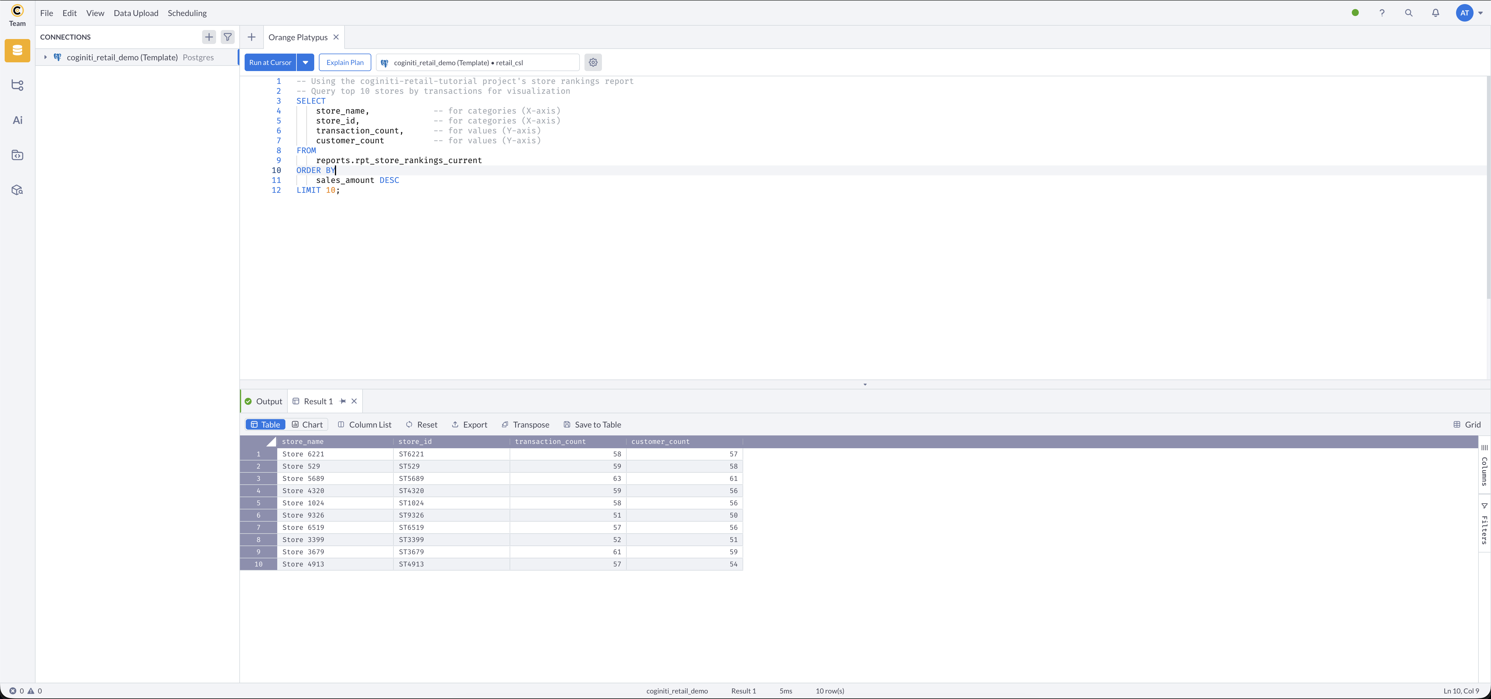
Example Query:

-- Using the coginiti-retail-tutorial project's store rankings report
-- Query top 10 stores by transactions for visualization
SELECT
    store_name,             -- for categories (X-axis)
    store_id,               -- for categories (X-axis)
    transaction_count,      -- for values (Y-axis)
    customer_count          -- for values (Y-axis)
FROM
    reports.rpt_store_rankings_current
ORDER BY
    sales_amount DESC
LIMIT 10;

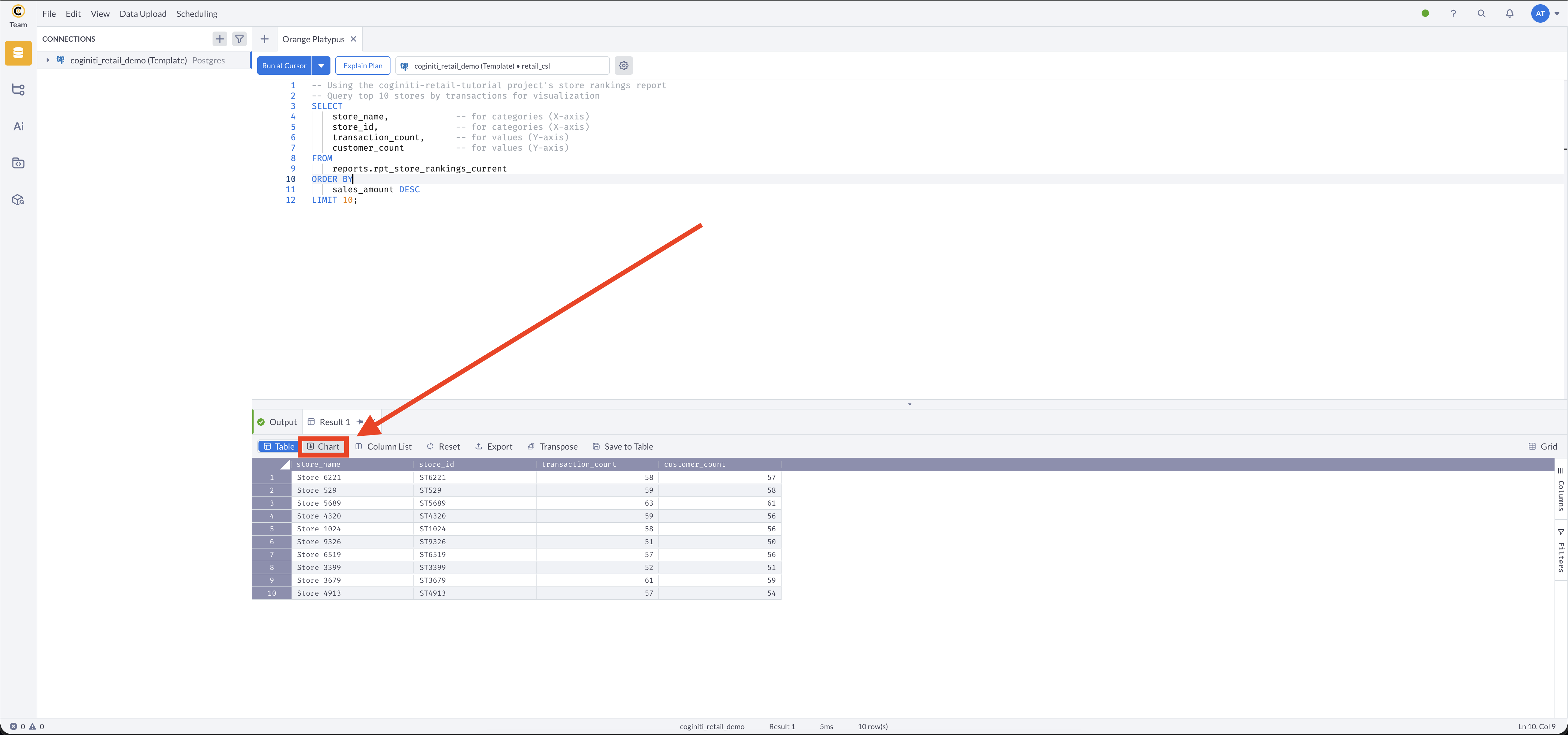
Step 2: Access the Charts Feature

1. After running your query, locate the query results grid
2. Look for the Charts button in the results toolbar
3. Click the Charts button to open the chart panel

Step 3: View and Interact with Your Chart

Your chart will appear with interactive features:

• Zoom: Use mouse wheel or zoom controls
• Restore: Return to the original view
• Show mini map: Click and drag to move to select some specific part of data in the chart
• Download: Export chart as PNG or export underlying data.
• Hover: See detailed values by hovering over data points
• Legend: Click legend items to show/hide series

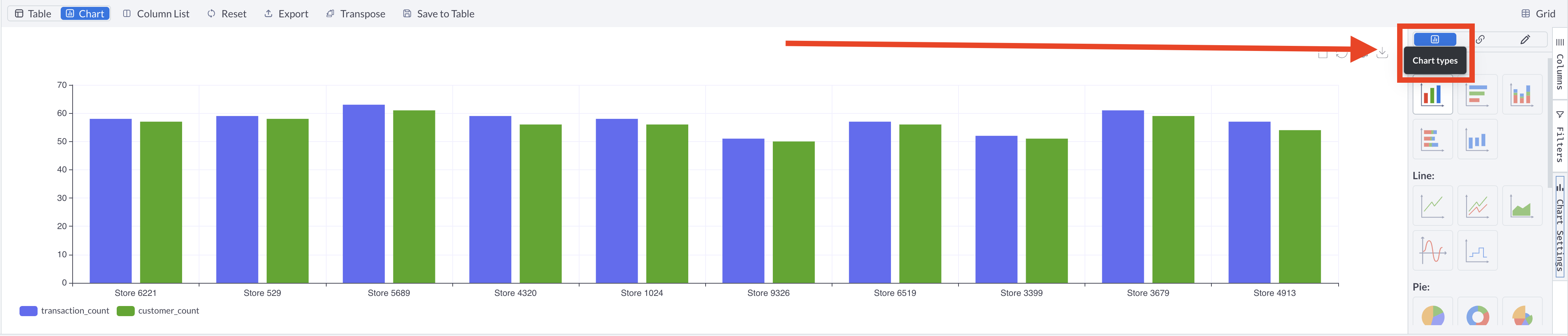
In the right panel click on Chart Settings button to open panel where you will see 3 tabs:

• Chart Types: Choose needed from the list of available chart types
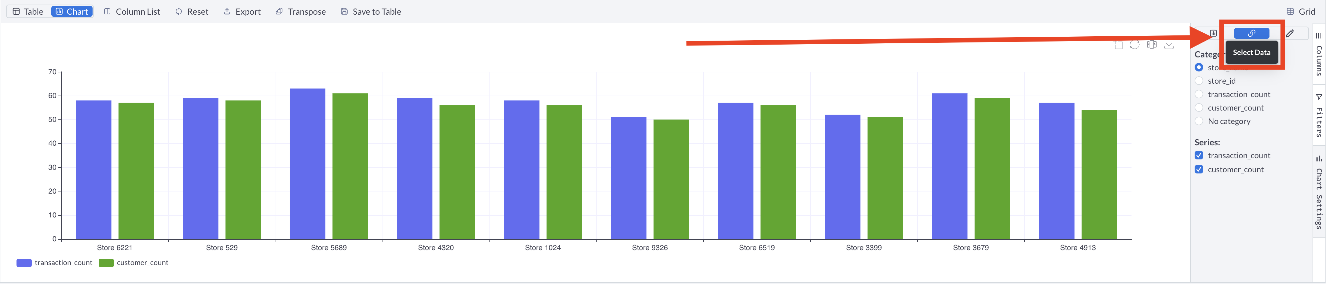
• Select Data: Choose needed Category of Series to show on chart
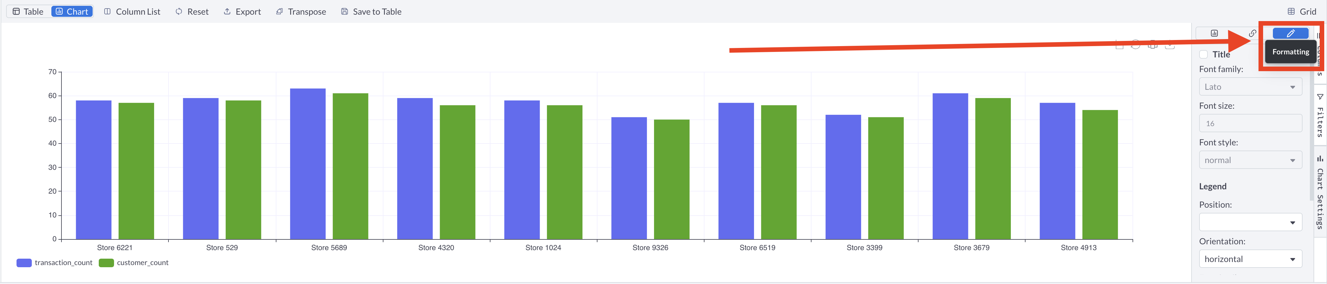
• Formatting: Add result tab name as name for the chart, change its format, as well as legend's format.

info

For more complete Chart Settings guide go to
Using the Chart Settings Panel

Chart Types

Bar Charts

Best for: Comparing categories, showing rankings, displaying discrete data

Data Requirements:

• At least one categorical column (X-axis)
• One or more numeric columns (Y-axis)

When to Use Bar Charts:

• Few categories (less than 10-15) for clarity
• Short category names that fit well on the X-axis
• Ranking data where order matters

Configuration Tips:

• Category names appear on the X-axis (bottom)
• Values extend vertically from bottom to top

Required Data Structure:

• Your query results must include at least one categorical column and one numeric column.

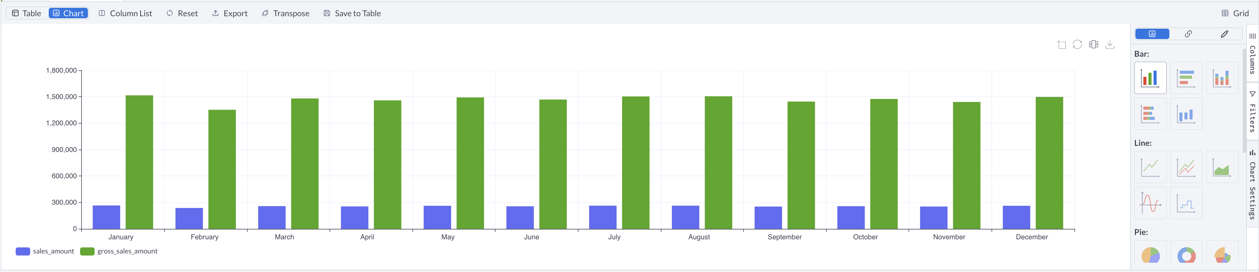
Example: Monthly Sales Comparison

-- Using retail project's mart layer for monthly sales trends
SELECT
    TO_CHAR(TO_TIMESTAMP(TO_CHAR(d.calendar_month, '99'), 'MM'), 'Month') AS calendar_month,
    SUM(f.sales_quantity) AS sales_amount,
    SUM(f.gross_sales_amount) AS gross_sales_amount
FROM
    mart.sale_return_fact f
INNER JOIN
    mart.date_dimension d
    ON d.date_key = f.transaction_date_key
WHERE
    d.calendar_year = 2022
GROUP BY
    d.calendar_month
ORDER BY
    d.calendar_month;

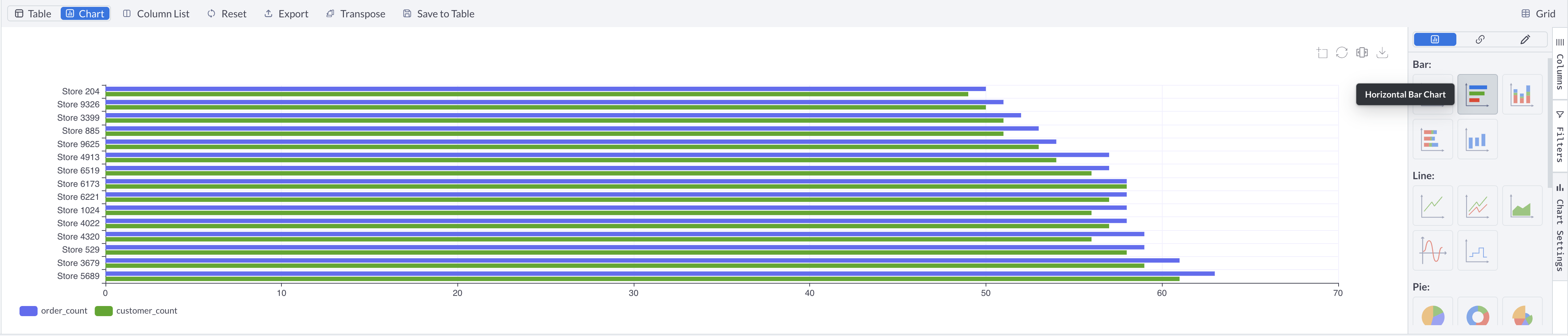
Horizontal Bar Charts

Best for: Comparing categories with long names, displaying rankings when category labels are lengthy

Data Requirements:

• At least one categorical column (Y-axis labels)
• One or more numeric columns (X-axis values)

When to Use Horizontal Bar Charts:

• Long category names that don't fit well on vertical charts
• Many categories (more than 10-15) for better readability
• Mobile-friendly displays where horizontal space is limited
• Comparison emphasis when you want to highlight value differences

Configuration Tips:

• Category names appear on the Y-axis (left side)
• Values extend horizontally from left to right
• Better for displaying large numbers of categories without crowding

Required Data Structure:

• Your query results must include at least one categorical column and one numeric column.

Example: Store Rankings by Transactions Volume

-- Using retail project's store rankings report (ideal for long store names)
SELECT
    store_name,
    transaction_count as order_count,
    customer_count
FROM
    reports.rpt_store_rankings_current
WHERE
    store_rank <= 15
ORDER BY
    transaction_count DESC;

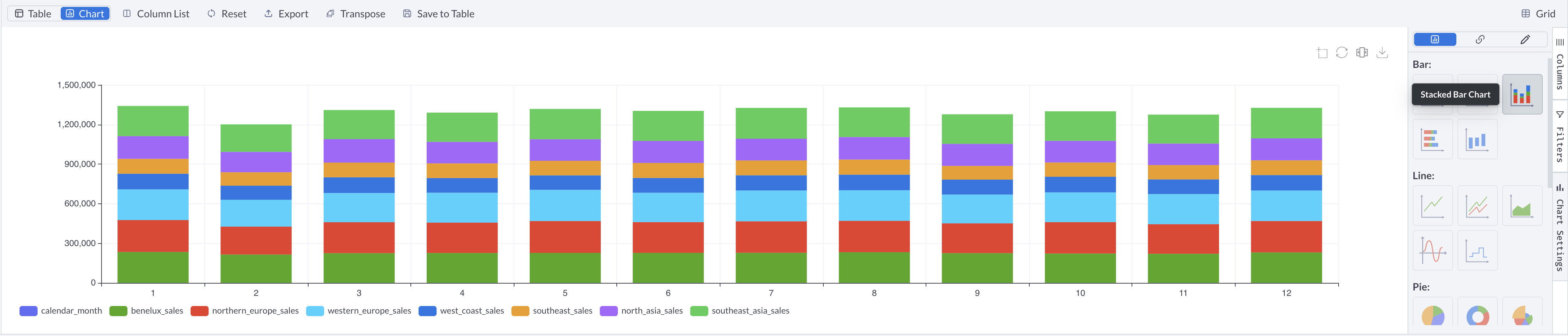
Stacked Bar Charts

For bar charts, choose stacked version to show individual values within overall category:

Vertical Stacked Bar Charts

1. Select "Stacked Bar Chart" from chart types
2. Multiple series will stack vertically on top of each other
3. Shows individual values over the category
4. Ideal for showing individual values simultaneously for multiple categories

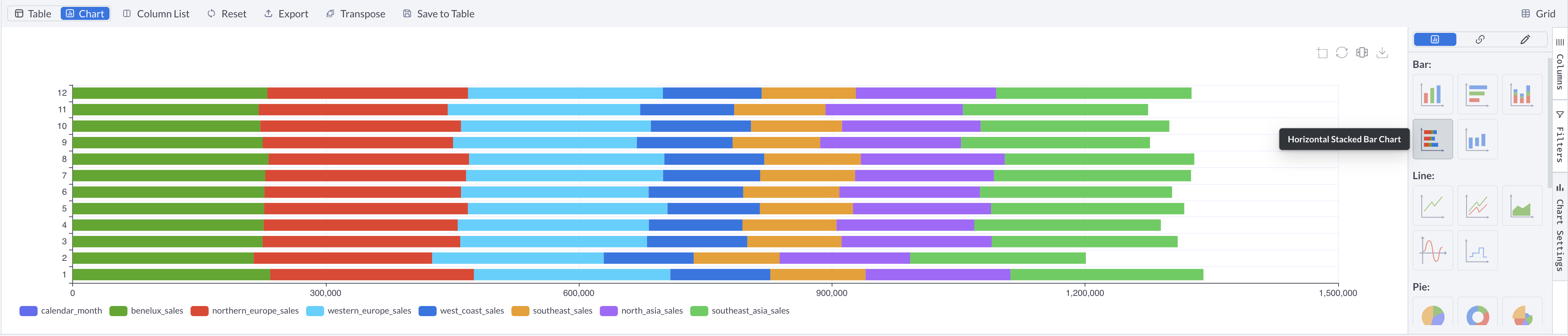
Horizontal Stacked Bar Charts

1. Select "Horizontal Stacked Bar Chart" from chart types
2. Multiple series stack horizontally from left to right
3. Combines benefits of horizontal layout with stacking visualization
4. Best for:
   • Long category names with multiple data series
   • Composition analysis where you want to show parts of the total
   • Mobile displays with limited vertical space
   • Many categories that benefit from horizontal orientation

Configuration Tips for Stacked Charts:

• Ensure data series have meaningful relationships for stacking
• Consider the order of stacking - place most important series at the bottom
• Use effective naming to help users interpret stacked segments

Example: Sales Composition by Market Area

-- Using retail mart layer to show market area breakdown over time
SELECT
    TO_CHAR(TO_TIMESTAMP(TO_CHAR(d.calendar_month, '99'), 'MM'), 'Month') AS calendar_month,
    SUM(CASE WHEN b.market_area_name = 'Benelux' THEN f.gross_sales_amount ELSE 0 END) as benelux_sales,
    SUM(CASE WHEN b.market_area_name = 'Northern Europe' THEN f.gross_sales_amount ELSE 0 END) as northern_europe_sales,
    SUM(CASE WHEN b.market_area_name = 'Western Europe' THEN f.gross_sales_amount ELSE 0 END) as western_europe_sales,
    SUM(CASE WHEN b.market_area_name = 'West Coast' THEN f.gross_sales_amount ELSE 0 END) as west_coast_sales,
    SUM(CASE WHEN b.market_area_name = 'Southeast' THEN f.gross_sales_amount ELSE 0 END) as southeast_sales,
    SUM(CASE WHEN b.market_area_name = 'North Asia' THEN f.gross_sales_amount ELSE 0 END) as north_asia_sales,
    SUM(CASE WHEN b.market_area_name = 'Southeast Asia' THEN f.gross_sales_amount ELSE 0 END) as southeast_asia_sales
FROM
    mart.sale_return_fact f
LEFT JOIN 
    mart.date_dimension d
    ON d.date_key = f.transaction_date_key
LEFT JOIN 
    mart.business_unit_dimension b
    ON f.business_unit_key = b.business_unit_key
WHERE
    d.calendar_year = 2022
GROUP BY
    d.calendar_month
ORDER BY
    d.calendar_month;

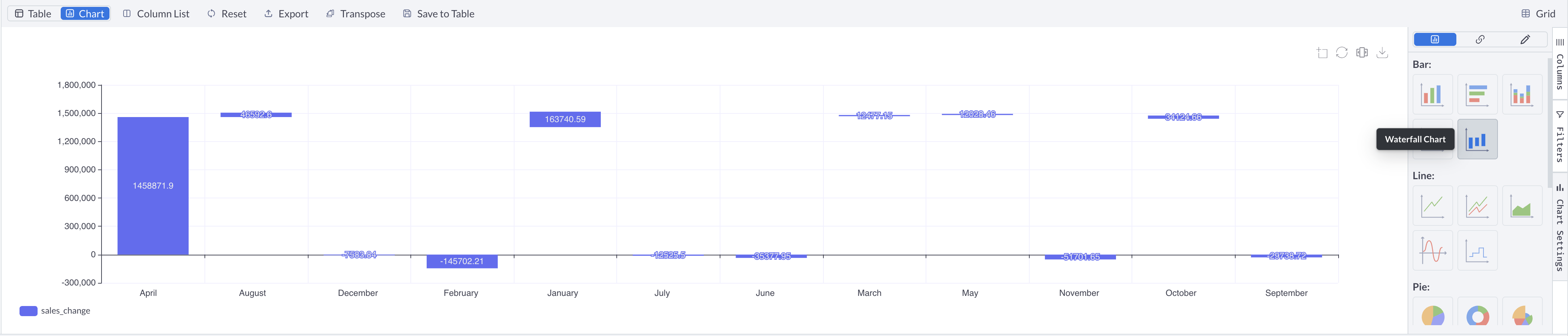
Waterfall Charts

Best for: Showing cumulative effects of sequential changes

Data Requirements:

• One categorical column (X-axis)
• One numeric column (Y-axis)
• At least 10 data points for meaningful trends
• Use when you want to illustrate how an initial value is affected by a series of intermediate positive or negative values leading to a final value
• Ideal for financial data, profit/loss analysis, and step-by-step changes
• Ensure data includes both increases and decreases for a complete waterfall effect

Required Data Structure:

• Your query results must include at least one categorical column and one numeric column.

Example: Monthly Revenue Changes

-- Using retail mart layer to calculate month-over-month changes
WITH monthly_sales AS (
    SELECT
        TO_CHAR(TO_TIMESTAMP(TO_CHAR(d.calendar_month, '99'), 'MM'), 'Month') AS calendar_month,
        SUM(f.gross_sales_amount) as month_sales
    FROM
        mart.sale_return_fact f
    INNER JOIN
        mart.date_dimension d
        ON d.date_key = f.transaction_date_key
    WHERE
        d.calendar_year = 2022
    GROUP BY
        TO_CHAR(TO_TIMESTAMP(TO_CHAR(d.calendar_month, '99'), 'MM'), 'Month')
)
SELECT
    calendar_month,
    month_sales - LAG(month_sales, 1, 0) OVER (ORDER BY calendar_month) as sales_change
FROM
    monthly_sales
ORDER BY
    calendar_month;

Line Charts

Best for: Showing trends over time, continuous data

Data Requirements:

• One time/sequence column (X-axis)
• One or more numeric columns (Y-axis)
• At least 10 data points for meaningful trends

When to Use Line Charts:

• Time series data to show trends over days, months, or years
• Continuous data where values change smoothly
• Multiple series to compare trends across categories
• Highlighting changes over intervals

Configuration Tips:

• Use date/time columns for X-axis for best results
• Choose Smooth Line Chart or Step Line Chart for most preferable view for you

Required Data Structure:

• Your query results must include at least one date/time column and one or more numeric columns.

Example: Daily Sales Trend

-- Using retail project's daily snapshot report for time series visualization
SELECT
    sale_date as transaction_date,
    transaction_count as daily_transactions,
    unique_customers as daily_unique_customers,
    unique_stores as daily_unique_stores
FROM
    reports.rpt_daily_snapshot_current
ORDER BY
    sale_date;

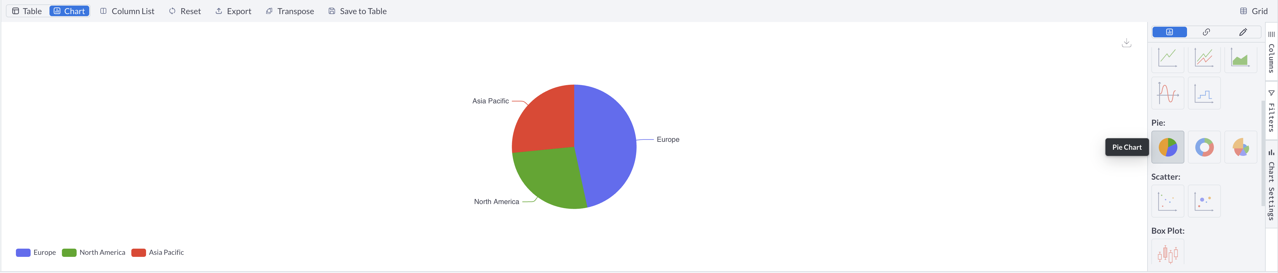
Pie Charts

Best for: Showing parts of a whole, composition analysis

Data Requirements:

• One categorical column for segments
• One numeric column for values
• Works best with fewer than 10 segments
• Avoid very small segments for clarity

When to Use Pie Charts:

• Few categories (ideally less than 6) for clear visualization
• Emphasizing proportions of a whole
• Single series data to avoid confusion
• Highlighting key segments that make up significant portions

Required Data Structure:

• Your query results must include one categorical column and one numeric column.

Example: Market Share by Region

-- Using retail mart layer for regional sales analysis
SELECT
    bu.market_region_name as region_name,
    SUM(f.gross_sales_amount) as total_sales
FROM
    mart.sale_return_fact f
INNER JOIN 
    mart.business_unit_dimension bu
    ON bu.business_unit_key = f.business_unit_key
INNER JOIN 
    mart.date_dimension d
    ON d.date_key = f.transaction_date_key
WHERE
    d.calendar_year = 2022
GROUP BY
    bu.market_region_name
ORDER BY
    total_sales DESC;

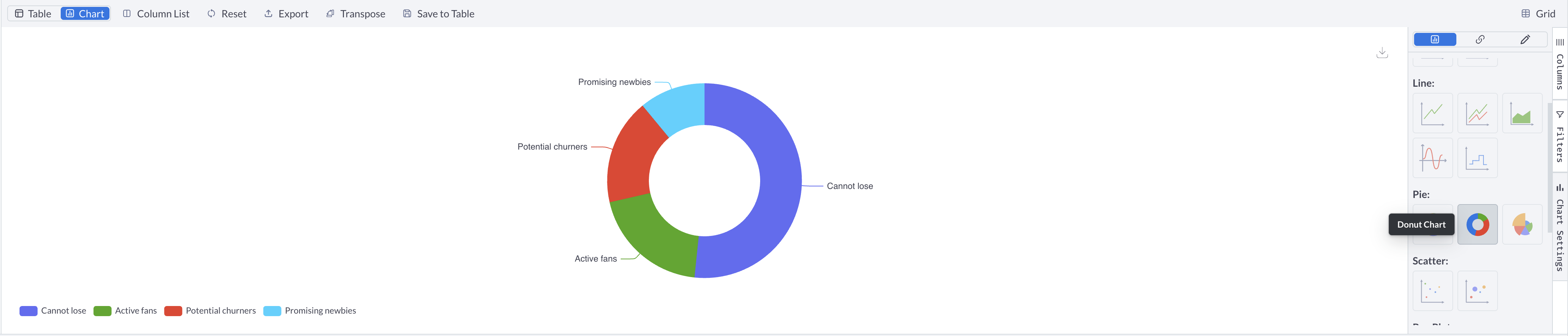
Donut Charts

Best for: Similar to pie charts, with a focus on aesthetics and space for labels

Data Requirements:

• One categorical column for segments
• One numeric column for values
• Works best with fewer than 10 segments
• Avoid very small segments for clarity

Required Data Structure:

• Your query results must include one categorical column and one numeric column.

Example: Customer Segment Distribution

-- Using retail mart layer with RFM segmentation
SELECT
    rfm_segment as customer_segment,
    COUNT(DISTINCT persona_key) as customer_count
FROM
    mart.persona_derived_attributes
WHERE
    rfm_segment IS NOT NULL
    AND rfm_segment != 'Other'
GROUP BY
    rfm_segment
ORDER BY
    customer_count DESC;

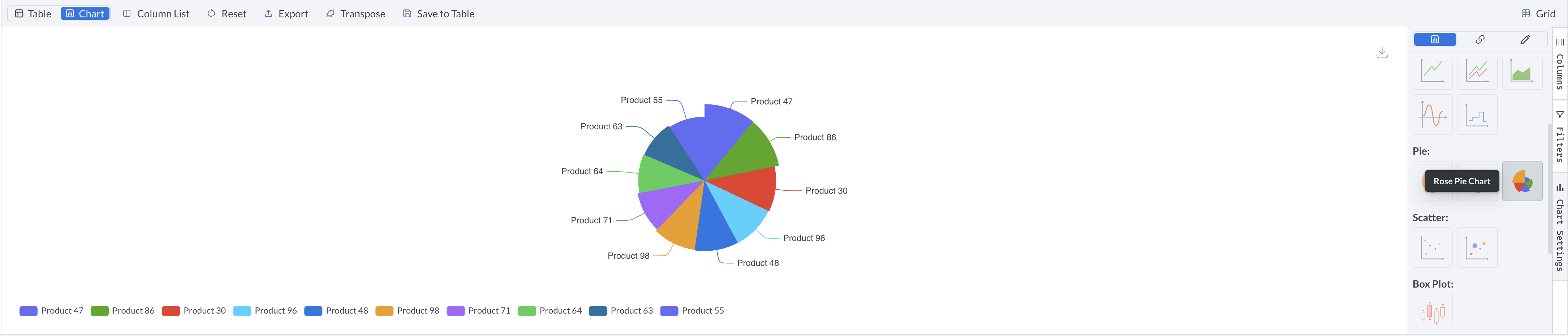
Rose Pie Charts

Best for: Emphasizing differences in segment sizes with variable radius

Data Requirements:

• One categorical column for segments
• One numeric column for values
• Works best with fewer than 10 segments
• Avoid very small segments for clarity
• Use when you want to highlight magnitude differences more dramatically than standard pie charts

Required Data Structure:

• Your query results must include one categorical column and one numeric column.

Example: Product Category Sales Share

-- Using retail mart layer for product sales analysis
SELECT
    i.item_name,
    SUM(f.gross_sales_amount) as category_sales
FROM
    mart.sale_return_fact f
INNER JOIN 
    mart.item_dimension i
    ON i.item_key = f.item_key
INNER JOIN 
    mart.date_dimension d
    ON d.date_key = f.transaction_date_key
WHERE
    d.calendar_year = 2022
GROUP BY
    i.item_name
HAVING
    SUM(f.gross_sales_amount) > 0
ORDER BY
    category_sales DESC
LIMIT 10;

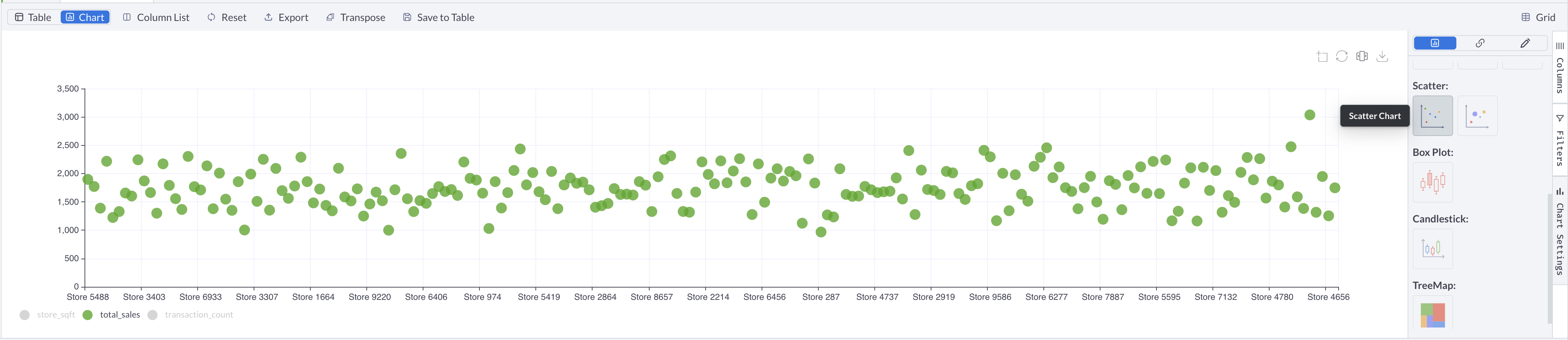
Scatter Charts

Best for: Showing correlations, relationships between variables

Data Requirements:

• Two numeric columns (X and Y coordinates)
• At least 20 data points for meaningful patterns

Required Data Structure:

• Your query results must include two numeric columns.

Example: Store Performance Analysis

-- Using retail mart layer to analyze store size vs performance correlation
SELECT
    bu.business_unit_name as store_name,
    bu.selling_area_size as store_sqft,
    SUM(f.gross_sales_amount) as total_sales,
    COUNT(DISTINCT f.transaction_id) as transaction_count
FROM
    mart.sale_return_fact f
INNER JOIN 
    mart.business_unit_dimension bu
    ON bu.business_unit_key = f.business_unit_key
INNER JOIN 
    mart.date_dimension d
    ON d.date_key = f.transaction_date_key
WHERE
    bu.selling_area_size IS NOT NULL
    AND d.calendar_year = 2022
GROUP BY
    bu.business_unit_name,
    bu.selling_area_size
HAVING
    COUNT(DISTINCT f.transaction_id) > 10
ORDER BY
    bu.selling_area_size
LIMIT 200;

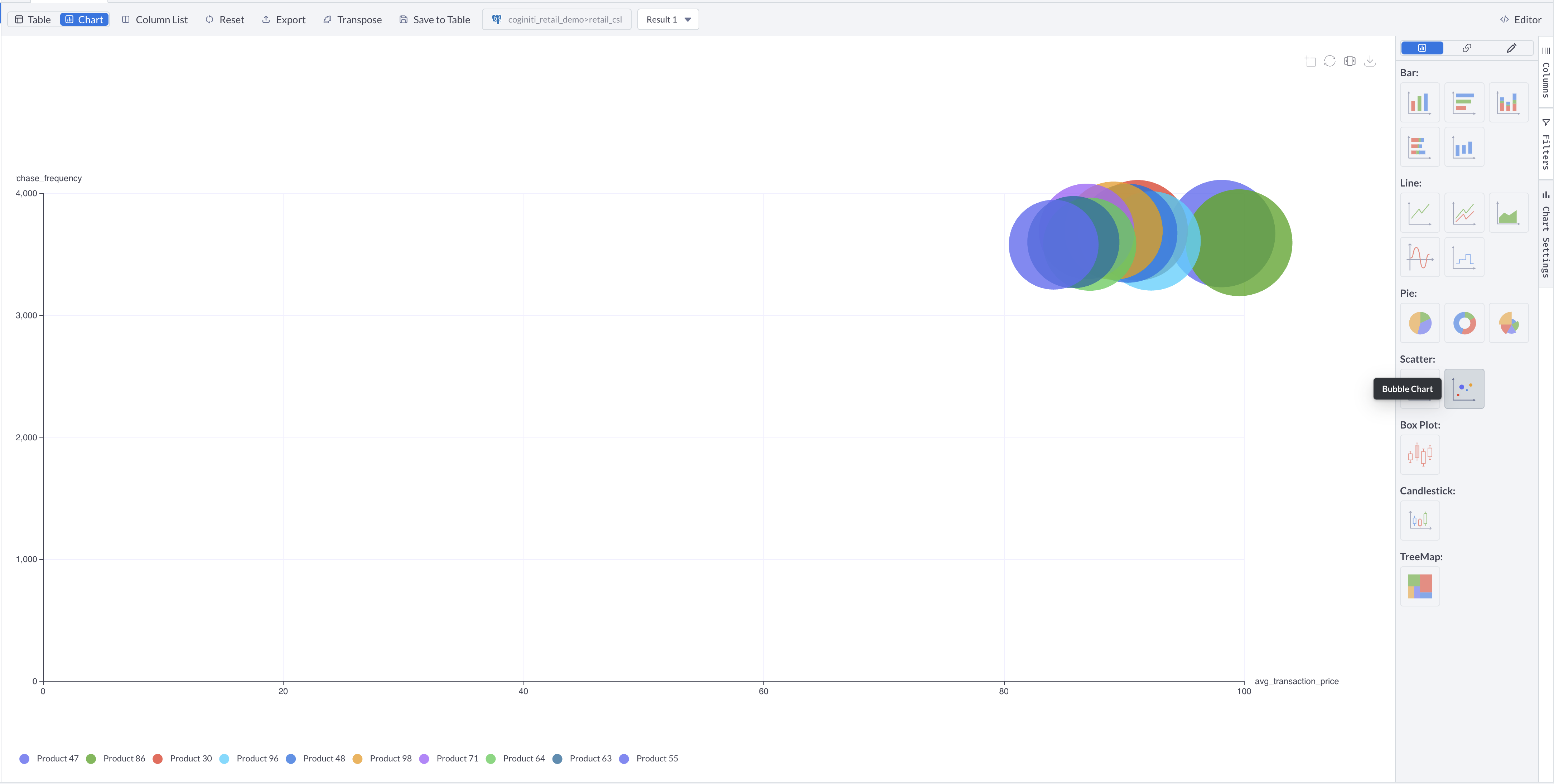
Scatter Bubble Charts

Best for: Showing correlations with an additional dimension (size)

Data Requirements:

• Two numeric columns (X and Y coordinates)
• Optional: Third column for bubble size
• At least 20 data points for meaningful patterns
• Use when you want to visualize relationships between two variables while also representing a third variable through bubble size

Required Data Structure:

• Your query results must include at least two numeric columns and optionally a third numeric column for bubble size.

Example: Customer Lifetime Value Analysis

-- Using retail mart layer to analyze product price vs sales frequency
-- Bubble size represents total revenue contribution
SELECT
    i.item_name as product_name,
    ROUND(AVG(f.gross_sales_amount), 2) as avg_transaction_price,
    COUNT(DISTINCT f.transaction_id) as purchase_frequency,
    SUM(f.gross_sales_amount) as total_revenue,
    SUM(f.sales_quantity) as units_sold
FROM
    mart.sale_return_fact f
INNER JOIN 
    mart.item_dimension i
   ON i.item_key = f.item_key
INNER JOIN 
    mart.date_dimension d
   ON d.date_key = f.transaction_date_key
WHERE
    d.calendar_year = 2022
GROUP BY
    i.item_name
HAVING
    COUNT(DISTINCT f.transaction_id) >= 10
ORDER BY
    total_revenue DESC
LIMIT 10;

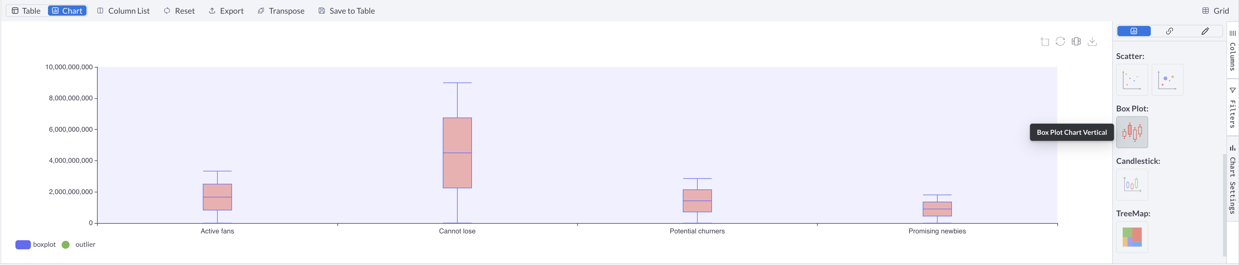
Box Plot Charts

Best for: Statistical distribution, outliers, quartiles

Data Requirements:

• One categorical column (X-axis)
• One numeric column (Y-axis)
• Multiple numeric columns for multiple box plots
• At least 5 data points per box plot
• Minimum of 20 total data points for meaningful statistics

Box Plot Interpretation:

Box Elements:

• Bottom of Box: First quartile (Q1, 25th percentile)
• Middle Line: Median (Q2, 50th percentile)
• Top of Box: Third quartile (Q3, 75th percentile)

Analysis Insights:

• Box Height: Shows interquartile range (data spread)
• Median Position: Indicates data skewness
• Whisker Length: Shows data range and potential outliers

Example: Sales Distribution by Market Region

-- Using retail mart layer to analyze spending patterns across customer segments
-- Firstly - change ROW COUNT LIMIT to 0 in the tab settings ! ! !
SELECT
    da.rfm_segment as customer_segment,
    f.transaction_id,
    SUM(f.gross_sales_amount) as order_value
FROM
    mart.sale_return_fact f
INNER JOIN 
    mart.persona_dimension p
    ON p.persona_key = f.persona_key
INNER JOIN 
    mart.persona_derived_attributes da
    ON da.persona_key = p.persona_key
INNER JOIN 
    mart.date_dimension d
    ON d.date_key = f.transaction_date_key
WHERE
    d.calendar_year = 2022
    AND da.rfm_segment IS NOT NULL
    AND da.rfm_segment != 'Other'
GROUP BY
    da.rfm_segment,
    f.transaction_id
HAVING
    SUM(f.gross_sales_amount) > 0
ORDER BY
    da.rfm_segment,
    order_value;

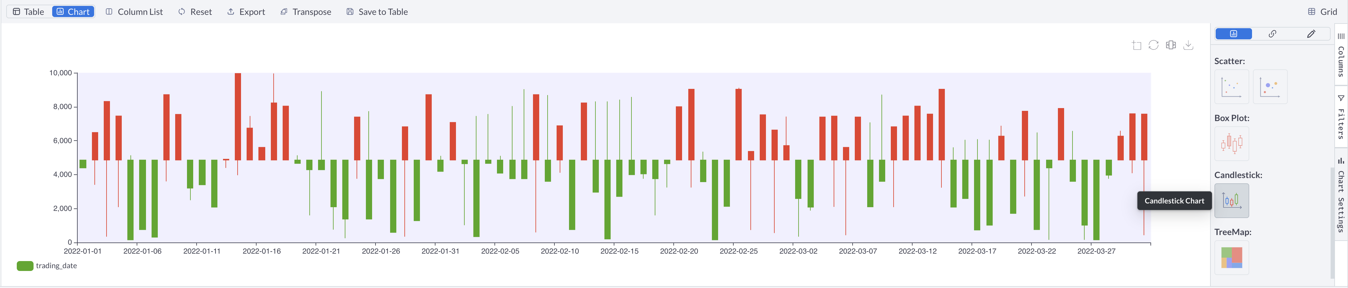
Candlestick Charts

Best for: Financial data, showing open/high/low/close values

Data Requirements:

• One time/sequence column (X-axis)
• Four numeric columns: open, high, low, close
• At least 10 data points for meaningful trends

warning

Required Data Structure: Your query results must include these specific columns (names may very) in particular order:

SELECT 
    date_column,        -- Time dimension (X-axis)
    open_value,         -- Opening value
    high_value,         -- Highest value in period
    low_value,          -- Lowest value in period
    close_value         -- Closing value
FROM 
    your_table
ORDER BY 
    date_column;

Example: Daily Sales Performance

-- Using retail mart layer with aggregated daily metrics for candlestick visualization
-- Firstly - change ROW COUNT LIMIT to 0 in the tab settings ! ! !
WITH daily_sales AS (
    SELECT
        d.business_day_date as trading_date,
        MIN(f.gross_sales_amount) as daily_low,
        MAX(f.gross_sales_amount) as daily_high,
        FIRST_VALUE(f.gross_sales_amount) OVER (PARTITION BY d.business_day_date ORDER BY f.transaction_datetime) as opening_sales,
        LAST_VALUE(f.gross_sales_amount) OVER (PARTITION BY d.business_day_date ORDER BY f.transaction_datetime ROWS BETWEEN UNBOUNDED PRECEDING AND UNBOUNDED FOLLOWING) as closing_sales
    FROM
        mart.sale_return_fact f
    INNER JOIN 
        mart.date_dimension d
        ON d.date_key = f.transaction_date_key
    WHERE
        d.calendar_year = 2022
        AND d.calendar_month <= 3
    GROUP BY
        d.business_day_date,
        f.transaction_datetime,
        f.gross_sales_amount
)
-- Putting our columns in the needed order
SELECT DISTINCT
    trading_date,       -- Time dimension (X-axis)
    opening_sales,      -- Opening value
    daily_high,         -- Highest value in period
    daily_low,          -- Lowest value in period
    closing_sales       -- Closing value
FROM
    daily_sales
ORDER BY
    trading_date;

Candlestick Chart Interpretation:

• Green Candles: Close price higher than open price (bullish)
• Red Candles: Close price lower than open price (bearish)
• Wicks: Show the full range between high and low values
• Body Size: Indicates the difference between open and close values

Treemap Charts

Best for: Hierarchical data, showing relative sizes

Data Requirements:

• Hierarchical or nested categorical data
• Numeric values for sizing
• Works best up to 10 000 data points

When to Use Treemaps:

• Hierarchical data to show parts of a whole

Required Data Structure:

• Your query results must include at least one categorical column and one numeric column.

Example: Hierarchical Sales by Geography

-- Using retail mart layer with full location hierarchy for treemap visualization
SELECT
    bu.market_region_name as region_name,
    bu.market_area_name as area_name,
    bu.district_name,
    SUM(f.gross_sales_amount) as total_sales
FROM
    mart.sale_return_fact f
INNER JOIN mart.business_unit_dimension bu
    ON bu.business_unit_key = f.business_unit_key
INNER JOIN mart.date_dimension d
    ON d.date_key = f.transaction_date_key
WHERE
    d.calendar_year = 2022
GROUP BY
    bu.market_region_name,
    bu.market_area_name,
    bu.district_name
HAVING
    SUM(f.gross_sales_amount) > 0
ORDER BY
    bu.market_region_name,
    bu.market_area_name,
    bu.district_name,
    total_sales DESC;

Interactive Features

Interactive Data Control

Column Selection Panel

The sidebar panel provides comprehensive control over which data appears in your visualizations.

Selecting Columns for Visualization:

1. Open column selection panel in the chart sidebar
2. Review available columns from your query results
3. Check/uncheck columns to include or exclude from visualization
4. Observe real-time updates in both chart and data table
5. Fine-tune selection based on visual clarity and analysis needs

Column Selection Strategies:

• Focus on Key Metrics: Include primary measures essential for analysis
• Exclude noise columns that don't add analytical value
• Group related metrics for comparative visualization
• Progressive Analysis: Start with core dimensions and add complexity gradually

Real-time Filtering

Apply filters that simultaneously update both chart visualizations and underlying data tables for consistent analysis.

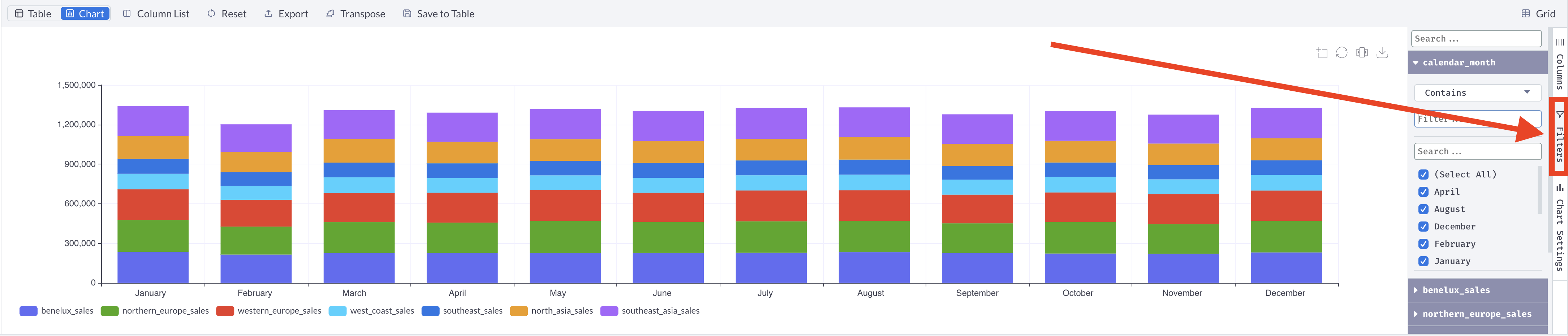
Filter Types Available:

• Range Filters: Numerical ranges for metrics and measures, date/time ranges for temporal analysis
• Category Filters: Multi-select options for dimensional data, include/exclude patterns
• Conditional Filters: Comparison operators, pattern matching, null/not null options

Applying Filters:

1. Access filter controls in the chart sidebar
2. Select filter type appropriate for your data column
3. Set filter criteria using available controls
4. Apply filter to see immediate updates in both chart and table
5. Adjust criteria as needed for optimal analysis focus

Data Consistency Across Views

Ensure that changes in chart configuration are reflected in tabular data views and vice versa.

Synchronized View Benefits:

• Analytical Confidence: Consistent data between visual and tabular representations
• Workflow Efficiency: Seamless transitions between chart and table analysis
• Quality Assurance: Cross-view validation and single source of truth

Using the Chart Settings Panel

The Chart Settings Panel is your control center for customizing charts. It appears on the right side when you create or edit a chart and contains three main tabs.

Accessing the Chart Settings Panel

1. Create a new chart or select an existing chart
2. The Chart Settings panel icon placed on the right sidebar
3. Click the Chart Settings icon to open it
4. The panel stays open while you work on your chart

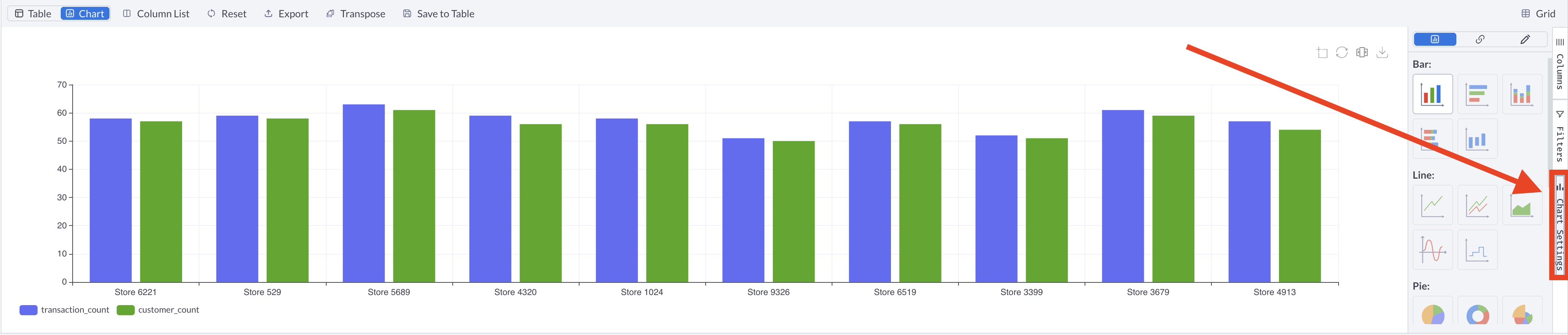
Chart Settings Panel Structure

The Chart Settings Panel has three main tabs, each represented by an icon:

Chart Types Tab (Chart icon):

• Select and switch between different chart types
• Preview available chart variations
• Instantly see how your data looks in different formats

Select Data Tab (Link icon):

• Configure which columns to use for your chart
• Map data to chart axes and series
• Control what data appears in your visualization

Formatting Tab (Edit icon):

• Customize the visual appearance of your chart
• Control titles, legends, fonts, and colors
• Fine-tune the chart's presentation

Using the Chart Types Tab

1. Browse Categories: Scroll through the organized chart type sections
2. Preview Charts: Hover over icons to see chart type names
3. Select Type: Click on any chart type icon to apply it immediately
4. Active Indicator: The currently selected chart type is highlighted
5. Instant Preview: Your chart updates immediately when you select a new type

Select Data Tab - Guide

The Select Data tab controls which columns from your dataset are used in the chart and how they're mapped to chart elements.

Category Section

The Category section determines what appears on the X-axis (or segments in pie charts):

1. Available Options: Shows all text and date columns from your data
2. Radio Button Selection: Choose one category column at a time
3. Column Preview: See the column name and data type
4. Automatic Selection: First suitable column is selected by default

Best Practices for Categories:

• Choose columns with distinct, meaningful values
• Use aggregated data for clarity
• Date columns work well for time-series data
• Text columns should have consistent formatting

Series Section

The Series section controls what numeric data is displayed (Y-axis values):

1. Multiple Selection: Use checkboxes to select multiple numeric columns
2. Column Information: Each checkbox shows the column name and data type
3. Active Indicators: Selected series are checked
4. Dynamic Updates: Chart updates immediately when you change selections

Best Practices for Series:

• Select 1-5 series for optimal readability
• Choose columns with similar value ranges when possible
• Mix different metrics (e.g., count + average) carefully
• Consider using separate charts for very different scales

Formatting Tab - Guide

The Formatting tab provides comprehensive control over your chart's visual appearance, organized into sections for different chart elements.

Title Formatting Section

Control the main chart title appearance:

1. Enable/Disable Toggle:

   • Use checkbox to show or hide the result tab / chart title
   • When disabled, other title options are grayed out

2. Font Family Selection:

   • Use dropdown to select font family from 9 available
   • Default: Lato (matches Coginiti's interface)

3. Font Size Control:

   • Enter numeric value for title font size
   • Typical range: 12-24 pixels

4. Font Style Options:

   • Choose from: Normal, Bold, Italic
   • Bold: Emphasizes the title (recommended)
   • Italic: Subtle emphasis
   • Normal: Clean, understated appearance

Legend Formatting Section

Customize how the chart legend appears and behaves:

1. Position Settings:

   • Choose from 6 positions: top-left, top-right, top-center, bottom-left, bottom-right, bottom-center
   • Top positions: Good for charts with horizontal space
   • Bottom positions: Traditional placement, works with most chart types
   • Left/Right: Best for charts with many series
   • Center positions: Clean, balanced appearance

2. Orientation Control:

   • Horizontal: Legend items arranged in rows (space-efficient)
   • Vertical: Legend items arranged in columns (easier to read with long names)
   • Choose based on available space and number of series

3. Font Customization:

   • Font Family: Same 9 options as title formatting
   • Font Size: Numeric input for legend text size (typically 10-16px)
   • Font Style: Normal, Bold, or Italic options
   • Keep consistent with chart title or use smaller size

Formatting Best Practices

1. Consistency:

   • Use the same font family throughout the chart
   • Maintain readable size relationships (title > legend > labels)
   • Stick to 1-2 font styles maximum

2. Readability:

   • Ensure sufficient contrast between text and background
   • Test formatting at different zoom levels
   • Consider the final display context (screen, print, presentation)

3. Professional Appearance:

   • Use bold titles for emphasis
   • Position legends to balance the overall layout
   • Choose fonts that match your organization's style guide

Best Practices for Effective Charts

Data Preparation Tips

1. Clean Your Data:

   • Remove null values or handle them appropriately
   • Ensure consistent data types
   • Sort data logically (by date, size, alphabetically)

2. Right-Size Your Dataset:

   • Limit to essential data points for clarity
   • Use aggregation for large datasets
   • Consider date ranges for time series data

3. Choose Appropriate Granularity:

   • Daily vs. monthly vs. yearly data
   • Individual items vs. grouped categories

Chart Selection Guidelines

1. Match Chart Type to Data Type:

   • Time series → Line charts
   • Categories → Bar charts
   • Composition → Pie charts
   • Correlation → Scatter charts

2. Consider Your Audience:

   • Executive dashboards: Simple, high-level charts
   • Analysis: Detailed, interactive charts
   • Presentations: Clear, focused visualizations

3. Optimize for Insight:

   • Highlight the most important data
   • Use colors to guide attention
   • Include context with titles and labels

Troubleshooting Common Issues

Chart Not Displaying

Possible Causes:

• No numeric data in selected columns
• All values are null or zero
• Browser compatibility issues

Solutions:

1. Check data types in your query results
2. Verify you have at least one numeric column
3. Try a different chart type
4. Refresh the page and try again

Chart Display Issues

Possible Causes:

• Too many data series selected
• Incompatible data types for selected chart type
• Overly complex data relationships

Solutions:

1. Reduce the number of series in the Select Data tab
2. Choose appropriate chart types for your data
3. Simplify data with aggregation functions (SUM, AVG, COUNT)
4. Use filters in your SQL query to focus on key data

Data Not Showing Correctly

Possible Causes:

• Incorrect column mapping
• Data type mismatches
• Null or invalid values

Solutions:

1. Verify X-axis and Y-axis column selections
2. Check for null values in your data
3. Ensure numeric columns are properly formatted
4. Review your SQL query for data issues

Performance Issues

Symptoms: Slow chart loading or interaction

Solutions:

1. Reduce data volume - Apply filters or aggregation in SQL
2. Simplify chart type - Use simpler charts for large datasets
3. Optimize query - Improve query performance for faster results
4. Check browser resources - Close other applications if needed

Chart-Specific Issues

Candlestick Chart Problems

Missing Candles:

• Verify OHLC columns are properly mapped
• Check for null values in required columns
• Ensure proper date/time ordering in data

Incorrect Price Display:

• Validate data ranges for realistic financial values
• Check decimal precision in numerical columns
• Verify currency conversion if applicable

Box Plot Problems

No Box Visible:

• Ensure sufficient data points for statistical calculations
• Check for data variance (constant values won't show boxes)
• Verify numerical data types for calculation columns

Excessive Outliers:

• Review data quality for potential errors
• Consider data transformation or filtering
• Adjust outlier sensitivity if configurable

Interactive Feature Issues

Filter Problems

Filters Not Working:

• Check filter compatibility with selected data types
• Verify filter syntax for pattern-based filters
• Confirm data synchronization is enabled
• Reset filters and reapply incrementally

Column Selection Problems

Column changes don't update visualizations:

• Refresh chart view to force update
• Check column data types for chart compatibility
• Verify column contains data (not all nulls)
• Reset column selection to defaults

tip

For more information about other exciting Coginiti features visit https://docs.coginiti.co/intro/

Thank you for choosing us!